
【力学】2重振り子の運動方程式の導出と数値シミュレーション【ラグランジュの運動方程式】【SymPy】
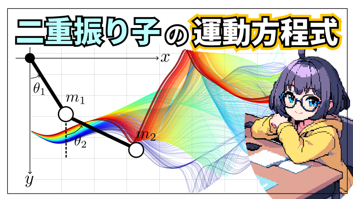
この記事では力学の基本やカオス理論で出てくる二重振り子の運動方程式をラグランジュの運動方程式を用いて導出します。
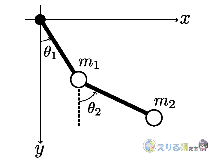
問題設定
以下の図のように、二重振り子は2つの振り子がつながった構造をしています。
質量の無視できる長さ \(L_1\) の棒の先に質点 \(m_1\) が取り付けられていて、棒は原点中心に回転できるとします。
同様に 質量の無視できる長さ \(L_2\) の棒の先に質点 \(m_2\) が取り付けられていて、棒は質点 \(m_1\)を中心に回転できるとします。
また、棒の回転角をそれぞれ下の図のように\(\theta_1,\ \theta_2\)とします。
運動方程式の導出
それでは一般化座標\(\theta_1,\ \theta_2\) に関するラグランジュの運動方程式を導出してみましょう。
とはいえ、ラグランジュの運動方程式の計算ってかなり大変ですよね。
そんなときはSymPyというPythonのライブラリを使えばパソコンが手計算を代わりにやってくれます。
SymPyとその使い方は以下の記事で説明しています。すごく便利なので、使ったことないよって方はこれを機に一度トライしてみてください!

テストでは手計算する必要があるので頼りすぎは良くないけどね。
質点の位置と速度
質点 \(m_1\) の位置を\((x_1,\ y_1)\)とすると、幾何学的関係から以下が成り立ちます。
$$
x_1 = L_1 \sin \theta_1
$$$$
y_1 = -L_1 \cos \theta_1
$$
質点 \(m_2\) の位置を\((x_2,\ y_2)\) は以下のように表されます。
$$
x_2 = L_1 \sin \theta_1 + L_2 \sin \theta_2
$$$$
y_2 = -L_1 \cos \theta_1 – L_2 \cos \theta_2
$$
それぞれ時間微分\((x_1,\ y_1)\)、\((x_2,\ y_2)\)をそれぞれ時間微分することで質点の速度になり、以下のように計算できます。
$$
\dot{x_1} = L_1 \cos \theta_1 \dot{\theta_1}
$$$$
\dot{y_1} = L_1 \sin \theta_1 \dot{\theta_1}
$$$$
\dot{x_2} = L_1 \cos \theta_1 \dot{\theta_1} + L_2 \cos \theta_2 \dot{\theta_2}
$$$$
\dot{y_2} = L_1 \sin \theta_1 \dot{\theta_1} + L_2 \sin \theta_2 \dot{\theta_2}
$$
運動エネルギーと位置エネルギー
次に、系全体(=質点1と2を合わせて考える)の運動エネルギーと位置エネルギーを計算します。
系全体の運動エネルギーを\(T\)とすると、
$$
T = \frac{1}{2} m_1 (\dot{x_1}^2 + \dot{y_1}^2) + \frac{1}{2} m_2 (\dot{x_2}^2 + \dot{y_2}^2)
$$
で表されます。これを先ほどの速度の式を用いて計算することで以下のように整理できます。
$$
T = \frac{1}{2} m_1 L_1^2 \dot{\theta_1}^2 + \frac{1}{2} m_2 [L_1^2 \dot{\theta_1}^2 + L_2^2 \dot{\theta_2}^2 + 2 L_1 L_2 \dot{\theta_1} \dot{\theta_2} \cos(\theta_1 – \theta_2)]
$$
系全体の位置エネルギーを\(U\)とします。保存力は重力のみなので\(U\)は以下のように与えられます。
$$
U = m_1 g y_1 + m_2 g y_2
$$
したがって、先ほどの位置の式を用いて計算することで以下のように整理できます。
$$
U = -m_1 g L_1 \cos \theta_1 – m_2 g (L_1 \cos \theta_1 + L_2 \cos \theta_2)
$$
ラグランジアン
ラグランジアン\(L\)は
$$
L = T – U
$$
で与えられます。先ほどの\(T,\ U\)を代入して整理すると以下のようになります。
$$
L = \frac{1}{2} m_1 L_1^2 \dot{\theta_1}^2 + \frac{1}{2} m_2 [L_1^2 \dot{\theta_1}^2 + L_2^2 \dot{\theta_2}^2 + 2 L_1 L_2 \dot{\theta_1} \dot{\theta_2} \cos(\theta_1 – \theta_2)]
$$$$
+ m_1 g L_1 \cos \theta_1 + m_2 g (L_1 \cos \theta_1 + L_2 \cos \theta_2)
$$
ラグランジュの運動方程式
\(\theta_i\) に関するラグランジュの運動方程式は以下のようになります。
$$
\frac{d}{dt} \left( \frac{\partial L}{\partial \dot{\theta_i}} \right) – \frac{\partial L}{\partial \theta_i} = 0
$$
まず、\(\theta_1\) に関する運動方程式から計算していきます。ラグランジュの運動方程式の各項は以下のように計算できます。
$$
\frac{\partial L}{\partial \theta_1} = -m_2 L_1 L_2 \dot{\theta_1} \dot{\theta_2} \sin(\theta_1 – \theta_2) – (m_1 + m_2) g L_1 \sin \theta_1
$$$$
\frac{\partial L}{\partial \dot{\theta_1}} = (m_1 + m_2) L_1^2 \dot{\theta_1} + m_2 L_1 L_2 \dot{\theta_2} \cos(\theta_1 – \theta_2)
$$$$
\frac{d}{dt} \left( \frac{\partial L}{\partial \dot{\theta_1}} \right) = (m_1 + m_2) L_1^2 \ddot{\theta_1} + m_2 L_1 L_2 \ddot{\theta_2} \cos(\theta_1 – \theta_2)
$$$$
– m_2 L_1 L_2 \dot{\theta_2} \sin(\theta_1 – \theta_2) (\dot{\theta_1} – \dot{\theta_2})
$$
したがって、\(\theta_1\) に関する運動方程式は以下のようになります。
$$
(m_1 + m_2) L_1^2 \ddot{\theta_1} + m_2 L_1 L_2 \ddot{\theta_2} \cos(\theta_1 – \theta_2)\ \ \ \ \ \ \ \ \ \ \ \ \ \ \ \ \ \ \ \ \ \ \ \ \ \ \ \ \ \ \ \ \ \
$$$$
+ m_2 L_1 L_2 \dot{\theta_2}^2 \sin(\theta_1 – \theta_2) + (m_1 + m_2) g L_1 \sin \theta_1 = 0
$$
次に、\(\theta_2\) に関する運動方程式から計算します。ラグランジュの運動方程式の各項は以下のように計算できます。
$$
\frac{\partial L}{\partial \theta_2} = m_2 L_1 L_2 \dot{\theta_1} \dot{\theta_2} \sin(\theta_1 – \theta_2) – m_2 g L_2 \sin \theta_2
$$$$
\frac{\partial L}{\partial \dot{\theta_2}} = m_2 L_2^2 \dot{\theta_2} + m_2 L_1 L_2 \dot{\theta_1} \cos(\theta_1 – \theta_2)
$$$$
\frac{d}{dt} \left( \frac{\partial L}{\partial \dot{\theta_2}} \right) = m_2 L_2^2 \ddot{\theta_2} + m_2 L_1 L_2 \ddot{\theta_1} \cos(\theta_1 – \theta_2) – m_2 L_1 L_2 \dot{\theta_1} \sin(\theta_1 – \theta_2) (\dot{\theta_1} – \dot{\theta_2})
$$
したがって、\(\theta_2\) に関する運動方程式は以下のようになります。
$$
m_2 L_2^2 \ddot{\theta_2} + m_2 L_1 L_2 \ddot{\theta_1} \cos(\theta_1 – \theta_2) – m_2 L_1 L_2 \dot{\theta_1}^2 \sin(\theta_1 – \theta_2) + m_2 g L_2 \sin \theta_2 = 0
$$
数値シミュレーションで運動方程式を解く
先ほど導出した一般化座標\(\theta_1,\ \theta_2\) に関するラグランジュの運動方程式を解いてみましょう。
解くといっても、この方程式は解析的に解くことはできないので、数値積分を使って運動方程式を解きます。
解析的に解くとは、微積分や代数などの数学的な手法を用いて、解を厳密な関数として表現することです。
今回はPythonを使って微分方程式を解いてみようと思います。Scipyに入っているodeintという関数を使って微分方程式を解きます。
解くときに作ったPythonスクリプトは以下の通りです。コピペしたらそのまま使用できるので、ぜひ自分でも解いてみてください。
import os
import numpy as np
from scipy.integrate import odeint
import matplotlib.pyplot as plt


# 2重振り子の運動方程式を定義する関数
def double_pendulum_equations(state, t, L1, L2, m1, m2, g):
    theta1, z1, theta2, z2 = state

    c = np.cos(theta1 - theta2)
    s = np.sin(theta1 - theta2)

    a = (m1 + m2) * L1**2
    b = m2 * L1 * L2 * c
    c_val = m2 * L1 * L2 * c
    d_val = m2 * L2**2

    r1 = -m2 * L1 * L2 * z2**2 * s - (m1 + m2) * g * L1 * np.sin(theta1)
    r2 = m2 * L1 * L2 * z1**2 * s - m2 * g * L2 * np.sin(theta2)

    det = a * d_val - b * c_val

    if det == 0:
        z1_dot = 0
        z2_dot = 0
    else:
        z1_dot = (d_val * r1 - b * r2) / det
        z2_dot = (a * r2 - c_val * r1) / det

    return [z1, z1_dot, z2, z2_dot]


def save_figure(figure_object, filename):
    """
    Saves a Matplotlib figure object to a file.

    Args:
        figure_object (matplotlib.figure.Figure): The figure object to save.
        filename (str): The name of the file to save the figure as.
    """
    try:
        figure_object.savefig(filename, dpi=300)
        print(f"Figure saved successfully to {filename}")
    except Exception as e:
        print(f"An error occurred while saving the figure: {e}")


# パラメータの設定
L1 = 1.0
L2 = 1.0
m1 = 1.0
m2 = 1.0
g = 9.81

# 時間ステップの設定 (変更なし)
t_start = 0
t_end = 15
num_steps = 1000
t = np.linspace(t_start, t_end, num_steps)

# 初期値
theta1_0 = np.pi * 2 / 3
z1_0 = 0.0
theta2_0 = np.pi * 2 / 3
z2_0 = 0.0

state0 = [theta1_0, z1_0, theta2_0, z2_0]
s_ = odeint(double_pendulum_equations, state0, t, args=(L1, L2, m1, m2, g))

# 状態変数のプロット
ifig = -1
figname = []
ff = []

ifig += 1
figname.append("theta1")
ff.append(plt.figure(figsize=(16, 9), tight_layout=True))
ax = ff[ifig].add_subplot(111)
ax.plot(t, s_[:, 0], "-")
ax.set_xlabel("Time [s]")
ax.set_ylabel(r"$\theta_1$ [rad]")
ax.grid()

ifig += 1
figname.append("theta2")
ff.append(plt.figure(figsize=(16, 9), tight_layout=True))
ax = ff[ifig].add_subplot(111)
ax.plot(t, s_[:, 2], "-")
ax.set_xlabel("Time [s]")
ax.set_ylabel(r"$\theta_2$ [rad]")
ax.grid()

ifig += 1
figname.append("theta1dot")
ff.append(plt.figure(figsize=(16, 9), tight_layout=True))
ax = ff[ifig].add_subplot(111)
ax.plot(t, s_[:, 1], "-")
ax.set_xlabel("Time [s]")
ax.set_ylabel(r"$\dot{\theta_1}$ [rad/s]")
ax.grid()

ifig += 1
figname.append("theta2dot")
ff.append(plt.figure(figsize=(16, 9), tight_layout=True))
ax = ff[ifig].add_subplot(111)
ax.plot(t, s_[:, 3], "-")
ax.set_xlabel("Time [s]")
ax.set_ylabel(r"$\dot{\theta_2}$ [rad/s]")
ax.grid()


dirname = "simple_analysis"
os.makedirs(dirname, exist_ok=True)
for f_, n_ in zip(ff, figname):
    save_figure(f_, os.path.join(dirname, n_))

plt.show()
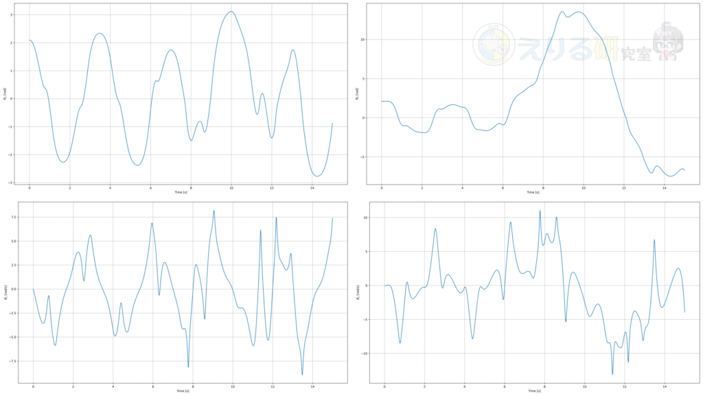
例えば、以下の初期条件
$$
\theta_1 = \theta_2 = \frac{2}{3}\pi
$$$$
\dot{\theta}_1 = \dot{\theta}_2 = 0
$$
のもとで解くと、各状態変数(\(\theta_1,\ \theta_2,\ \dot{\theta}_1,\ \dot{\theta}_2 \))の時間軌跡は以下のようになります。
これだけではあまり面白くないので、\(\theta_1,\ \theta_2\) の初期値を\(10^{-8}\) rad刻みでずらして1000パターンシミュレーションしてみましょう。
そのときの各状態変数(\(\theta_1,\ \theta_2,\ \dot{\theta}_1,\ \dot{\theta}_2 \))の時間軌跡は以下のようになります。
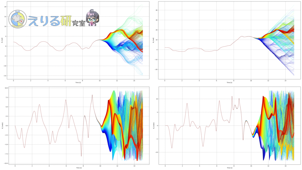
初期値に少しの差しか与えていないので最初は1000パターンとも同じ挙動を示しますが、ある時を境にまったく違う挙動になっていることがわかると思います。
ほんの少しの初期状態の差が二重振り子の運動に大きな影響を与えているということになります。
これは二重振り子の未来の状態を初期状態から予測することができないことを意味しています。
このような挙動をカオスと呼び、これを詳しく研究する分野をカオス理論といいます。
まとめ
この記事では力学の基本やカオス理論で出てくる二重振り子の運動方程式をラグランジュの運動方程式を用いて導出しました。
また、数値シミュレーションを用いて運動方程式を解いて、解の挙動を図示してみました。
二重振り子は力学を勉強すると必ず出てくる基本的な運動の一つでありながら、カオスが現れたりして奥が深いので、ぜひ皆さんも学んでみてください。
えりるさんは以下の教科書で力学の基本を勉強しました。大学生・力学初心者向けの教科書で、力学を学ぶ上で必要な数学的知識のフォローも基礎的なところからされているので読みやすかったです。

UGREENの Bluetoothトランスミッター& レシーバー です。イヤホンジャックに刺すとBluetooth非対応製品でもBluetoothを使えるようになって、ワイヤレスイヤホンなどを接続できるようになるって代物です。
えりるさんはこれを飛行機で使っています。
映画を見たりするときに、配られる有線イヤホンではなく自分のワイヤレスイヤホンを使えるようになります。手持ちのノイズキャンセリングイヤホンを使えるのが最高で、フライトが快適になりました。
注意点はLEDが少し眩しいので、100均で売ってる真っ黒のマスキングテープをボタンに貼って使っています。(これは絶対貼ったほうがいいので、本体色は黒がおすすめです)
